


7. Compensating for variable water depth to improve mapping of underwater habitats: why it is necessary
Editor: Dr Alasdair.J.Edwards, University of Newcastle, UK.
Aim of Lesson
To learn how to carry out 'depth-invariant' processing in order to compensate for the effect of light attenuation in the water column (i.e. water depth) on bottom reflectance using a CASI airborne image.
Learning Objectives
- To understand the concepts underlying depth-invariant processing.
- To inspect an unprocessed image using transects to discover how depth dominates returns from the seabed.
- To learn how to carry out depth-invariant processing of a CASI airborne image.
- To compare false colour composites of the processed and unprocessed images to see the results of compensating for the effects of water depth.
In this lesson two bands of an 8-waveband Compact Airborne Spectrographic Imager (CASI) image are used to introduce depth invariant processing. The image was recorded from a local Cessna at a spatial resolution of approx. 1 m2, near South Caicos Island in July 1995.
How to download the lesson
|
|
Concepts underlying depth-invariant processingWhen light penetrates water, its intensity decreases exponentially with increasing depth. The rate of attenuation differs with the wavelength. The red part of the visible spectrum attenuates more rapidly than shorter wavelength blue light and infrared light hardly penetrates water at all. The spectral radiances recorded by a sensor are therefore dependent both on the reflectance of the substrata and on the depth of the water. The influence of depth on the signal will create considerable confusion when attempting to map habitats. Since most marine habitat mapping exercises are only concerned with mapping benthic features, it is useful to remove the confounding influence of variable water depth. This lesson describes a fairly straightforward means of compensating for variable depth, which is applicable to clear waters such as those surrounding coral reef environments. | |
|
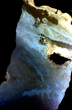
Right: Raw colour composite (bands 2, 3 and 4) of a CASI image of Cockburn Harbour with an automatic linear stretch. Note how the water steadily darkens from the shore (north of image) to the deeper reef at around 18 m depth at the south (bottom) end of the image. |
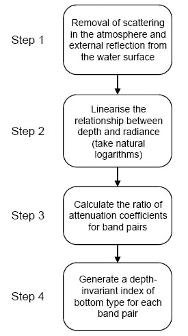
Correcting for water depthTo compensate for the depth involves four steps.
|
|
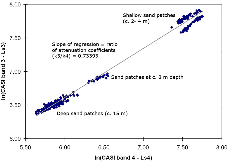
Above: Calculating the ratio of attenuation coefficients for CASI bands 3 and 4 using a series of coral sand patches at different depths. To linearise the relationship between depth and radiance the natural logarithms of the radiances in the CASI bands have been taken. The quantities Ls3 and Ls4 are the mean deepwater radiances in each band - 2 standard deviations.
|
|
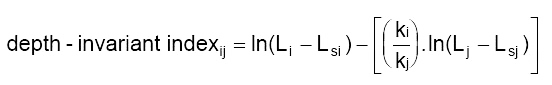
Implementing the calculations in BilkoThe equation to generate one depth-invariant band from each band-pair is simple to implement as a Bilko formula document:
where Ln is the natural logarithm, Lsi and Lsj are the mean deepwater radiances in bands i and j, and ki/kj is the ratio of their attenuation coefficients as determined from sand patches at varying depth. | |
|
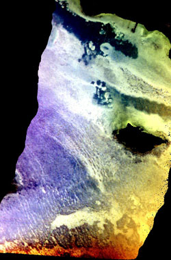
Left: Colour composite of three depth-invariant bands (bands 2/4, 3/4 and 3/5) of the CASI image of Cockburn Harbour with an automatic linear stretch. Note how the effect of water depth has been compensated for with the reef structure at 18 m depth at the south (bottom) end of the image now clearly visible. |
References
Lyzenga, D.R. 1978. Passive remote sensing techniques for mapping water depth and bottom features. Applied Optics 17 (3): 379-383.
Lyzenga, D.R. 1981. Remote sensing of bottom reflectance and water attenuation parameters in shallow water using aircraft and Landsat data. International Journal of Remote Sensing 2: 71-82.
Mumby, P.J., Clark, C.D., Green, E.P., and Edwards, A.J. 1998. Benefits of water column correction and contextual editing for mapping coral reefs. International Journal of Remote Sensing 19: 203-210.
 Previous: Lesson 6
|
Last update: 20 August 2018 | Contact |  |
Site Policy |
Next: Lesson 8

|