


4. Radiometric correction of satellite images: when and why radiometric correction is necessary
Author: Dr Alasdair J.Edwards, University of Newcastle, UK.
Aim of Lesson
To develop your understanding of concepts underlying radiometric correction and how to carry out the radiometric correction of satellite imagery, using two Landsat Thematic Mapper images obtained at different seasons under different atmospheric conditions as examples.
Learning Objectives
- To understand the difference between DN values, radiance, irradiance and reflectance.
- To understand why radiometric correction of imagery is required if (i) you are mapping changes in habitat or other features, or (ii) you are using more than one image in a study.
- To demonstrate how different atmospheric conditions can affect DN values by comparing these in two Landsat TM images acquired during different seasons.
- To understand the basic concepts behind atmospheric correction algorithms.
- To learn how to carry out the process of radiometric correction of two Landsat TM images obtained in different seasons and compare the resultant reflectance values.
How to download the lesson
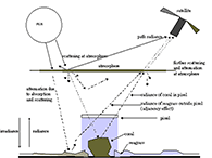
Figure 1. How atmospheric scattering contributes to the radiance measured at the top of the atmosphere. Larger figure
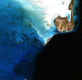
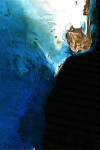
Figure 2. Colour composite of Landsat Thematic Mapper image of the South Caicos area of the Caicos Bank. Bands #3, #2 and #1 displayed through red, green and blue channels respectively. Larger image
Why you need radiometric correction
Digital sensors record the intensity of electromagnetic radiation (ER) from each spot viewed on the Earth's surface as a digital number (DN) for each spectral band. The DN values recorded by a sensor are proportional to upwelling ER (spectral radiance), the true units of which are W m-2 sr1 μm-1.
The spectral signature of a habitat (say mangrove) is not transferable if measured in digital numbers. The values are image specific; that is, they are dependent on the viewing geometry of the satellite, sun angle, Earth-Sun distance (which varies seasonally), specific weather conditions, and so on, at the moment the image was taken. It is in general far more useful to convert the DN values to spectral radiances.
However, the spectral radiances obtained from the calibration only account for the spectral radiance measured at the satellite sensor. By the time ER is recorded by a satellite or airborne sensor, it has already passed through the Earth's atmosphere twice (sun to target and target to sensor - see figure 1).
Atmospheric correction uses models (e.g. 5S and 6S models) to attempt to account for the effects of the atmosphere on the signal recorded so that spectral radiances at the satellite can be converted to at surface reflectances.
Lesson overview
This lesson uses two Landsat-5 Thematic Mapper images of the Turks and Caicos Islands, one taken during the northern winter (November) when conditions were relatively clear (see colour composite to right), and one taken during the summer (June) when conditions were much more hazy.
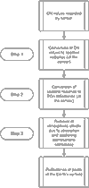
Figure 3. Flow chart showing the main steps i the lesson.
Larger figure
Initially, you compare the raw DN values for 5 pixels (in different habitats) between the two images in band #2 (green) and discover that the average difference between the DN values is almost 30% of their mean value. After radiometric and atmospheric correction of the two images, you find that the average difference between the surface reflectances of the same 5 pixels is less than 1% of their mean value.
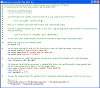
The radiometric correction process is broken down into three manageable steps (figure 3), each of which is explained in detail before you are asked to carry it out using a formula document For each step you are given a template formula document with a few lines that you need to complete (see example below in figure 5).
The first step is to use metadata provided with the image to convert the DN values to spectral radiances at the satellite using a formula document.
The second step converts the spectral radiance to top-of-atmosphere reflectances using data on the sun-angle at the time the image was taken (part of image metadata - figure 4), mean solar exoatmospheric irradiance (amount of light from the Sun reaching the satellite), and information on how to calculate the Earth-Sun distance for the date of acquisition.
The third step uses the outputs of a 5S (Simulation of the Satellite Signal in the Solar Spectrum) model to remove the effects of atmospheric scattering and absorption and derive surface reflectances for each pixel in each waveband.
|
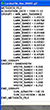
Figure 4. shows an example of metadata in the image's information pane. LMAX, LMIN and BANDWIDTH values are used in conversion of DN values to spectral radiances (Step 1). SUN_ELEVATION is used in conversion of spectral radiances to top-of-atmosphere reflectances (Step 2). |
Figure 5. Example template formula document for converting DN values to spectral radiances. Introduces use of image metadata in formulas. Here the user needs to complete constant lists marked "?????" with correct metadata attribute names. Larger image and explanation (pop-up) |
)
)
References
EOSAT 1993. Fast Format Document for TM Digital Products. Version B, Effective November 1, 1993. 10 pp.
Green, E.P., Mumby, P.J., Edwards, A.J. and Clark, C.D. (Ed. A.J. Edwards) (2000). Remote Sensing Handbook for Tropical Coastal Management. Coastal Management Sourcebooks 3. UNESCO, Paris. ISBN 92-3-103736-6 (paperback).
Kaufman, Y.J. 1989. The atmospheric effect on remote sensing and its correction. In Asrar, G. (ed.) Theory and Applications of Optical Remote Sensing. John Wiley and Sons.
Mather, P.M. 1999. Computer Processing of Remotely-Sensed Images: An Introduction. Second Edition. John Wiley and Sons. (Sections 4.4-4.6, pp. 87-94).
Moran, M.S., Jackson, R.D., Clarke, T.R., Qi, J. Cabot, F., Thome, K.J. and Markham, B.L. 1995. Reflectance factor retrieval from Landsat TM and SPOT HRV data for bright and dark targets. Remote Sensing of Environment 52: 218-230.
Price, J.C. 1987. Calibration of satellite radiometers and the comparison of vegetation indices. Remote Sensing of Environment 21: 15-27.
Tanré, D., Deroo, C., Dahaut, P., Herman, M. and Morcrette, J.J. 1990. Description of a computer code to simulate the satellite signal in the solar spectrum: the 5S code. International Journal of Remote Sensing 11 (4): 659-668.
Vermote, E. F., Tanré, D., Deuzé, J. L., Herman, M. and Morcrette, J. J. 1997. Second simulation of the satellite signal in the solar spectrum, 6S: an overview. IEEE Transactions on Geoscience and Remote Sensing 35: 675-686.
 Previous: Lesson 3
|
Last update: 20 August 2018 | Contact |  |
Site Policy |
Next: Lesson 5

|