Mini-Lesson 2: Covariance, correlation matrices and interpreting PCA loadings

Lesson Aims:

To introduce you to principal components analysis (PCA). This lesson shows how PCA is carried out, how the covariance or correlation matrices are calculated and how to calculate the eigenvalues and the percentage of total variance accounted for by each principal component.

Objectives:

By the end of this mini-lesson you will have an understanding of the fundamentals of how PCA works and how you could construct covariance and correlation matrices using statistics derived from Bilko histograms and scattergrams. You will also have learnt how to use the PC loadings. You will use these to calculate both the PC bands themselves and the eigenvalues for each PC band and thus work out how much of the total variance of the original images is accounted for in each of the PC bands.

Download the lesson:

If you have already registered as a Bilko user you can download this lesson by entering your e-mail address in the box below. If you are new to Bilko please register first, using the link on the top menu bar.

Content Overview

Adjacent bands in multispectral images are often correlated, which implies redundancy in the data as some information is being repeated in different bands. Principal components analysis (PCA) defines the number of dimensions that are present in a data set and the principal axes of variability and generates principal component images that encompass this variability. Thus in a six band Landsat Thematic Mapper (TM) image of land cover you may be able to encompass over 95% of the variability of the data in the first 3 principal component (PC) images. A colour composite image made with these three PC images is thus likely to give you a much clearer picture of different land cover types than any combination of three of the original bands. This mini-lesson is for those wishing to understand the workings of PCA who have a solid maths background! Warning: Not for the faint-hearted!

Sample images:

A selection of images from this mini lesson are shown below.

Landsat colour composite image, Note how fields with different crops are clearly distinguished.

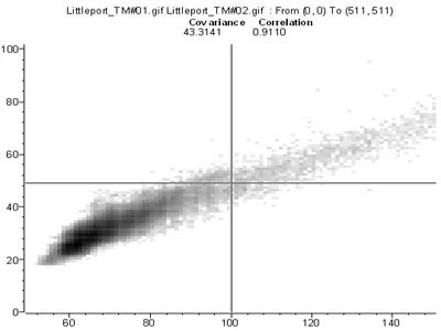
Scatter document showing the covariance and correlation in feature space between bands #1 (x-axis) and #2 (y-axis) of a Landsat Thematic Mapper image of the area around Littleport, near Ely in Cambridgeshire, UK. Note the close correlation (and thus redundancy of information) between the two wavebands.

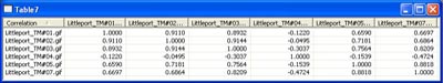
Correlation matrix for Principal Components Analysis of a 6 band Landsat Thematic Mapper image. Note how each band is perfectly correlated with itself (diagonal of 1.000 correlations) and how the table is symmetrical about the diagonal. Note also that the correlation between band#1 and band#2 is as shown in the scatter document.

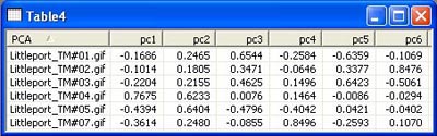
PC loadings table from a Principal Components Analysis of a 6 band Landsat TM image. Principal component 1 (pc1) will be -0.1686 x band#1 -0.1014 x band#2 -0.2204 x band#3 + 0.7675 x band#4 and so on down the column headed pc1.

Black and white pc1 image.

Colour composite image made up of pc1, pc2 and pc3 images. Note how fields with different crops are clearly distinguished. Almost 97% of the total variance in the 6 bands is accounted for by the first 3 principal components (pc1, pc2 and pc3 in the PC loadings table).